The decisionSupport function in the package requires two inputs:
1) a data table (.csv format) specifying the names and distributions for all uncertain variables
2) an R function that predicts decision outcomes based on the variables named in the data table
For this example, both inputs are provided to illustrate the process. Usually, data table and model have to be customized to fit the particulars of a specific decision.
The data table
The data table (wildfire_input_table.csv) contains all variables used in the model. Their distributions are described by a 90% confidence interval, which is specified by lower (5% quantile) and upper (95% quantile) bounds, as well as the shape of the distribution. This example uses four different distributions:
1) const – a constant value (not really a distribution)
2) norm – a normal distribution
3) tnorm_0_1 – a truncated normal distribution that can only have values between 0 and 1 (useful for probabilities; note that 0 and 1, as well as numbers outside this interval are not permitted as inputs)
4) posnorm – a normal distribution truncated at 0 (only positive values allowed)
For a full list of possible distributions, type ‘?random.estimate1d’ in R. When specifying confidence intervals for truncated distributions, note that approximately 5% of the random values should ‘fit’ within the truncation interval on either side. If there isn’t enough space, the function will generate a warning (usually it will still work, but the inputs may not look like you intended them to).
Default distributions are provided for all variables, but feel free to make adjustments by editing the .csv file in a spreadsheet program.
The decision model
Before you start developing the decision model, open R and download and load the decisionSupport package (version >1.102).
install.packages("decisionSupport")
library(decisionSupport)
You could simply start developing the decision model now, but since the model function will be designed to make use of variables provided to it externally (random numbers drawn according to the information in the data table), you’ll need to define sample values for all variables, if you want to test pieces of the code during the development process. This can be done manually, but it is more easily accomplished with the following helper function ‘make_variables’:
make_variables<-function(est,n=1)
{ x<-random(rho=est, n=n)
for(i in colnames(x)) assign(i,
as.numeric(x[1,i]),envir=.GlobalEnv)
}
(This function isn’t included in the decisionSupport package, because it places the desired variables in the global environment. This isn’t allowed for functions included in packages on R’s download servers.)
Applying make_variables to the data table (with default setting n=1) generates one random number for each variable, which then allows you to easily test code you’re developing:
filepath<-[folder, where the ‘wildfire_input_table.csv’ file is saved]
make_variables(estimate_read_csv(paste(filepath,
"wildfire_input_table.csv",sep="")))
You can now start developing the model, which has to be designed as a function for R, with the two arguments x and varnames, as well as a (named or unnamed) list of numbers as output:
[YOUR_MODEL]<-function(x,varnames)
{
[freely programmable content, relying only on inputs specified in the data table]
return(list([OUTPUTS]))
}
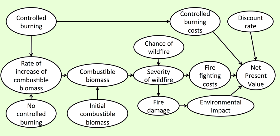
Below is an example model to calculate the Net Present Value (NPV) for the decision to manage forests with controlled burns:
controlled_burning<-function(x, varnames)
{
#simulate occurrence of fire (random event)
fire<-chance_event(fire_risk,value_if=1,n=n_years)
#set up time series vectors with one value for each simulation year
severe_fire_contr_burn<-rep(0,n_years)
severe_fire_no_burn<-rep(0,n_years)
env_imp_contr_burn<-rep(0,n_years)
env_imp_no_burn<-rep(0,n_years)
fire_fighting_cost_contr_burn<-rep(0,n_years)
fire_fighting_cost_no_burn<-rep(0,n_years)
#simulate occurrence of controlled burns (random event)
controlled_burns<-chance_event(controlled_burning_frequency,
value_if=1,n=n_years)
#calculate the change in the initial combustible biomass (Mg/ha)
biomass_contr_burn<-initial_biomass
biomass_no_burn<-initial_biomass
for(y in 2:n_years) #for all years but year one
{
if(controlled_burns[y])
biomass_contr_burn[y]<-biomass_after_burning*(1+
biomass_accumulation_rate_with_controlled_burning/100) else
biomass_contr_burn[y]<-biomass_contr_burn[y-1]*
(1+biomass_accumulation_rate_with_controlled_burning/100)
biomass_no_burn[y]<-biomass_no_burn[y-1]*
(1+biomass_accumulation_rate_without_controlled_burning/100)
#calculate the severity and impact of fire
if(fire[y])
{
#calculate when the accumulated combustible biomass (Mg/ha) that leads
# to severe fire is surpassed
if(biomass_contr_burn[y]>severity_threshold)
severe_fire_contr_burn[y]<-1
if(biomass_no_burn[y]>severity_threshold)
severe_fire_no_burn[y]<-1
#calculate the combustible biomass (Mg/ha) after a fire in a forest
# with controlled burning
if(severe_fire_contr_burn[y])
biomass_contr_burn[y]<-biomass_after_severe_fire else
biomass_contr_burn[y]<-biomass_after_mild_fire
#calculate the combustible biomass (Mg/ha) after a fire in a forest
# without controlled burning
if(severe_fire_no_burn[y])
biomass_no_burn[y]<-biomass_after_severe_fire else
biomass_no_burn[y]<-biomass_after_mild_fire
#calculate the environmental impact (USD) after a fire in a forest
# with controlled burning
if(severe_fire_contr_burn[y])
env_imp_contr_burn[y]<-env_imp_severe_fire else
env_imp_contr_burn[y]<-env_imp_mild_fire
#calculate the cost of wildfire (USD) in a forest with controlled
# burning
if(severe_fire_contr_burn[y])
fire_fighting_cost_contr_burn[y]<-
fire_fighting_cost_severe_fire else
fire_fighting_cost_contr_burn[y]<-
fire_fighting_cost_mild_fire
#calculate the environmental impact (USD) after a fire in a forest
# without controlled burning
if(severe_fire_no_burn[y])
env_imp_no_burn[y]<-env_imp_severe_fire else
env_imp_no_burn[y]<-env_imp_mild_fire
#calculate the cost of wildfire (USD) in a forest without controlled
# burning
if(severe_fire_no_burn[y])
fire_fighting_cost_no_burn[y]<-
fire_fighting_cost_severe_fire else
fire_fighting_cost_no_burn[y]<-
fire_fighting_cost_mild_fire
} #end of simulating severity and cost of fire
} #end of year loop
#calculate the cost (USD) of forest management through
# controlled burning and without controlled burning
costs_contr_burn<-
cost_of_controlled_burning*controlled_burns+
fire_fighting_cost_contr_burn
costs_no_burn<-fire_fighting_cost_no_burn
#calculate the bottom-line (USD) for forest management
# through controlled burning and without controlled burning
bottomline_contr_burn<-(-costs_contr_burn-env_imp_contr_burn)
bottomline_no_burn<-(-costs_no_burn-env_imp_no_burn)
#calculate the benefit of controlled burning over no
# controlled burning
benefit_of_controlled_burning<-
bottomline_contr_burn-bottomline_no_burn
#calculate the Net Present Value (NPV) for forest management
# with controlled burning
NPV_controlled_burning<-
discount(benefit_of_controlled_burning,discount_rate=discount_rate,
calculate_NPV=TRUE)
return(list(NPV_controlled_burning=NPV_controlled_burning))
}
Note that this model uses two ‘helper functions’ included in the decisionSupport package:
1) chance_event for determining whether an event occurs or not based on a specified probability
2) discount for adjusting net benefits for time preference (a standard economic practice). With the attribute calculate_NPV, the function automatically calculates the Net Present Value (the sum of discounted values)
Perform the Monte Carlo simulation with 10,000 model runs:
decisionSupport(
inputFilePath=paste(filepath,"wildfire_input_table.csv",
sep=""),
outputPath=paste(filepath,"MCResults",sep=""),
write_table=TRUE,
welfareFunction=controlled_burning,
numberOfModelRuns=10000,
functionSyntax="plainNames"
)
#the arguments are the following:
# inputFilePath = input file with estimates
# outputPath = output folder
# write_table = specifies whether all outputs should be saved as a table
# welfareFunction = the decision model function
# numberOfModelRuns = the number of model runs for the Monte
# Carlo simulation
# functionSyntax = technical parameter that allows specifying
# variables simply by the names given in the data table
# (otherwise a notation like x$[variable_name] would be needed)
This function produces a table of all inputs and outputs of the 10,000 model runs (mcSimulationResults.csv; only if write_table=TRUE), as well as two outputs for each model output variable:
1) a histogram showing all 10,000 output values
2) a variable-importance-plot that illustrates the sensitivity of model outputs to variation in each input variable (this is derived by statistically relating outputs to inputs using Projection-to-Latent-Structures (PLS) regression; results are also saved in a table)
All results are stored in the folder specified by outputPath. The two summary tables ‘mcSummary.csv’ and ‘welfareDecisionSummary.csv’ provide summaries of the results shown in the histogram.